Partial Dependence Plots

Partial dependence plots show the marginal effect one or two features have on the predicted outcome of a machine learning model. They work by calculating the average prediction of the model as one feature varies, while keeping all other features constant. Here’s a basic description of how PDPs are generated:

Choose a feature (or features) of interest for which you want to compute the PDP.
For each unique value of the chosen feature:
1. Change all instances of that feature in your dataset to that value, leaving all other features as they are.
2. Make predictions for this modified dataset and take the average of these predictions. This average prediction corresponds to the partial dependence of the chosen feature’s value.
Plot the unique feature values against the corresponding average predictions.

A PD plot can show whether the relationship between the target and a feature is linear, monotonic or more complex. For example, when applied to a linear regression model, partial dependence plots always show a linear relationship.

PDPs assume that the feature(s) being plotted are independent of the other features in the dataset. If this assumption is violated, the averages calculated for the partial dependence plot will include data points that are very unlikely or even impossible and this will make our plots unrealistic.

from pathlib import Path

import matplotlib.pyplot as plt
import numpy as np
import pandas as pd
from sklearn.datasets import fetch_openml, load_breast_cancer
from sklearn.ensemble import RandomForestClassifier
from sklearn.inspection import PartialDependenceDisplay
from sklearn.model_selection import train_test_split

pd.set_option("display.max_columns", None)

plt.rcParams["figure.facecolor"] = (1, 1, 1, 0)  # RGBA tuple with alpha=0
plt.rcParams["axes.facecolor"] = (1, 1, 1, 0)  # RGBA tuple with alpha=0

ROOT_DIR = Path.cwd().parent.parent

For classification where the machine learning model outputs probabilities, the partial dependence plot displays the probability for a certain class given different values for feature(s) in the dataset. An easy way to deal with multiple classes is to draw one line or plot per class.

data = load_breast_cancer()

X = pd.DataFrame(data.data, columns=data.feature_names)
y = pd.Series(data.target)

X_train, X_test, y_train, y_test = train_test_split(X, y, random_state=42)

clf = RandomForestClassifier(n_estimators=100, random_state=42)
clf.fit(X_train, y_train)
print(f"Accuracy on test data: {clf.score(X_test, y_test):.2f}")

Accuracy on test data: 0.97

X_train

	mean radius	mean texture	mean perimeter	mean area	mean smoothness	mean compactness	mean concavity	mean concave points	mean symmetry	mean fractal dimension	radius error	texture error	perimeter error	area error	smoothness error	compactness error	concavity error	concave points error	symmetry error	fractal dimension error	worst radius	worst texture	worst perimeter	worst area	worst smoothness	worst compactness	worst concavity	worst concave points	worst symmetry	worst fractal dimension
287	12.890	13.12	81.89	515.9	0.06955	0.03729	0.02260	0.01171	0.1337	0.05581	0.1532	0.4690	1.1150	12.68	0.004731	0.013450	0.016520	0.005905	0.01619	0.002081	13.620	15.54	87.40	577.0	0.09616	0.11470	0.11860	0.05366	0.2309	0.06915
512	13.400	20.52	88.64	556.7	0.11060	0.14690	0.14450	0.08172	0.2116	0.07325	0.3906	0.9306	3.0930	33.67	0.005414	0.022650	0.034520	0.013340	0.01705	0.004005	16.410	29.66	113.30	844.4	0.15740	0.38560	0.51060	0.20510	0.3585	0.11090
402	12.960	18.29	84.18	525.2	0.07351	0.07899	0.04057	0.01883	0.1874	0.05899	0.2357	1.2990	2.3970	20.21	0.003629	0.037130	0.034520	0.010650	0.02632	0.003705	14.130	24.61	96.31	621.9	0.09329	0.23180	0.16040	0.06608	0.3207	0.07247
446	17.750	28.03	117.30	981.6	0.09997	0.13140	0.16980	0.08293	0.1713	0.05916	0.3897	1.0770	2.8730	43.95	0.004714	0.020150	0.036970	0.011100	0.01237	0.002556	21.530	38.54	145.40	1437.0	0.14010	0.37620	0.63990	0.19700	0.2972	0.09075
210	20.580	22.14	134.70	1290.0	0.09090	0.13480	0.16400	0.09561	0.1765	0.05024	0.8601	1.4800	7.0290	111.70	0.008124	0.036110	0.054890	0.027650	0.03176	0.002365	23.240	27.84	158.30	1656.0	0.11780	0.29200	0.38610	0.19200	0.2909	0.05865
...	...	...	...	...	...	...	...	...	...	...	...	...	...	...	...	...	...	...	...	...	...	...	...	...	...	...	...	...	...	...
71	8.888	14.64	58.79	244.0	0.09783	0.15310	0.08606	0.02872	0.1902	0.08980	0.5262	0.8522	3.1680	25.44	0.017210	0.093680	0.056710	0.017660	0.02541	0.021930	9.733	15.67	62.56	284.4	0.12070	0.24360	0.14340	0.04786	0.2254	0.10840
106	11.640	18.33	75.17	412.5	0.11420	0.10170	0.07070	0.03485	0.1801	0.06520	0.3060	1.6570	2.1550	20.62	0.008540	0.023100	0.029450	0.013980	0.01565	0.003840	13.140	29.26	85.51	521.7	0.16880	0.26600	0.28730	0.12180	0.2806	0.09097
270	14.290	16.82	90.30	632.6	0.06429	0.02675	0.00725	0.00625	0.1508	0.05376	0.1302	0.7198	0.8439	10.77	0.003492	0.003710	0.004826	0.003608	0.01536	0.001381	14.910	20.65	94.44	684.6	0.08567	0.05036	0.03866	0.03333	0.2458	0.06120
435	13.980	19.62	91.12	599.5	0.10600	0.11330	0.11260	0.06463	0.1669	0.06544	0.2208	0.9533	1.6020	18.85	0.005314	0.017910	0.021850	0.009567	0.01223	0.002846	17.040	30.80	113.90	869.3	0.16130	0.35680	0.40690	0.18270	0.3179	0.10550
102	12.180	20.52	77.22	458.7	0.08013	0.04038	0.02383	0.01770	0.1739	0.05677	0.1924	1.5710	1.1830	14.68	0.005080	0.006098	0.010690	0.006797	0.01447	0.001532	13.340	32.84	84.58	547.8	0.11230	0.08862	0.11450	0.07431	0.2694	0.06878

426 rows × 30 columns

fig, ax = plt.subplots(ncols=3, nrows=10, figsize=(10, 25), constrained_layout=True)
display = PartialDependenceDisplay.from_estimator(clf, X_train, features=X_train.columns, kind="average", ax=ax)
plt.show()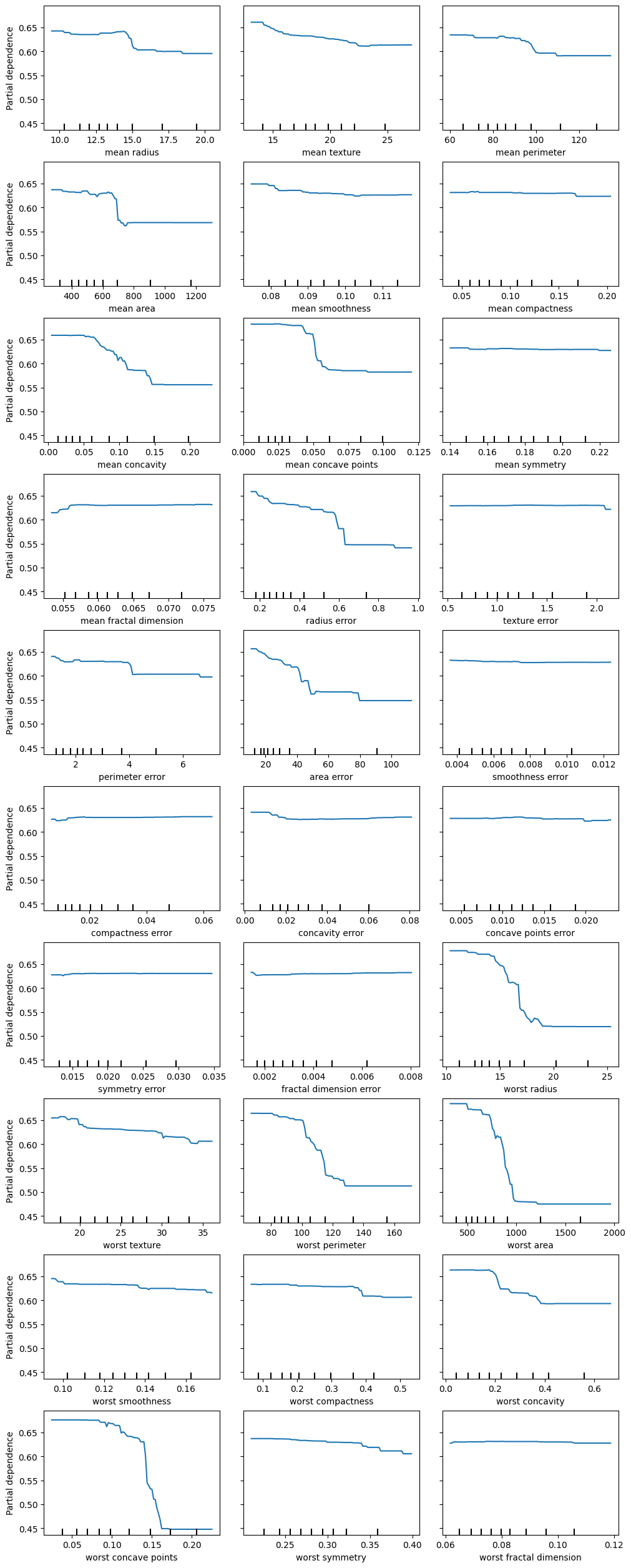

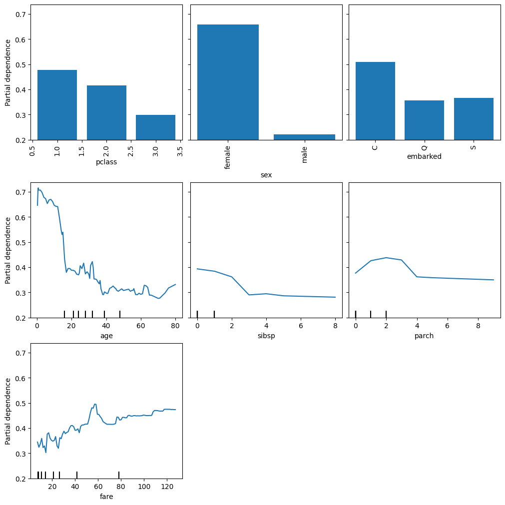
X, y = fetch_openml("titanic", version=1, as_frame=True, return_X_y=True, parser="pandas")

categorical_columns = ["pclass", "sex", "embarked"]
numerical_columns = ["age", "sibsp", "parch", "fare"]

X = X[categorical_columns + numerical_columns]
X_train, X_test, y_train, y_test = train_test_split(X, y, stratify=y, random_state=42)

from sklearn.pipeline import Pipeline
from sklearn.preprocessing import OrdinalEncoder
from sklearn.impute import SimpleImputer
from sklearn.compose import ColumnTransformer

categorical_encoder = OrdinalEncoder(handle_unknown="use_encoded_value", unknown_value=-1, encoded_missing_value=-1)
numerical_pipe = SimpleImputer(strategy="mean")

preprocessing = ColumnTransformer(
    [
        ("cat", categorical_encoder, categorical_columns),
        ("num", numerical_pipe, numerical_columns),
    ],
    verbose_feature_names_out=False,
)

rf = Pipeline(
    [
        ("preprocess", preprocessing),
        ("classifier", RandomForestClassifier(random_state=42)),
    ]
)
rf.fit(X_train, y_train)

print(f"RF train accuracy: {rf.score(X_train, y_train):.3f}")
print(f"RF test accuracy: {rf.score(X_test, y_test):.3f}")

RF train accuracy: 0.972
RF test accuracy: 0.787

display = PartialDependenceDisplay.from_estimator(
    rf, X_train, features=X_train.columns, kind="average", categorical_features=categorical_columns
)
display.figure_.set_size_inches(10, 10)
display.figure_.set_constrained_layout(True)
plt.show()